WEEK 1
Bullet Rigid Bodies
In the first week of this module, we learned about the Bullet system in Maya. We played around with the passive rigid body systems.
A rigid body is a polygonal or NURBS surface converted to an unyielding shape. Unlike conventional surfaces, rigid bodies collide rather than pass through each other during animation. To animate rigid body motion, you use fields, keys, expressions, rigid body constraints, or collisions with particles.
Scene Scale Tips:
Maya uses 1 unit to represent 1 centimeter. In simulations, 1 unit is 1metre.
The exercises and my process are presented below:

Exercise 1: Basic Usage of Bullett System
We need to make sure that we are using 25fps and playback speed is play every frame.
I have created a cube and a plane and played around with rigid body options. In order to make the cube interact with the plane when they collide, I set the cube to use the static body type and the plane to use the mesh static only.

Dominos
For the next exercise, we started by creating multiple cubes in the shape of a domino. We then made a chain of them falling, by using the bullet system.
I set the dynamic body type in order to make the fall realistic and I adjusted the velocity of the first domino.
Internal Fixed Frame Rate set to 240 Hz can improve solve quality.
Baking simulation = generates a single animation curve for an object whose actions are being provided by simulation rather than by keys and animation curves.
Further experimentation (Bullet on Domino's)
By using the MASH editor, I created again dominos. I have used the colour, curve, transform and dynamic nodes to set the colour of the dominos and also align them to a curve that I have manually made.

I then added a MASH Bulet Solver node where I then gave it the maximum internal frame rate and created a key frame for the first domino to hit another domino. Finally, I have adjusted the friction settings within the Bullet Solver and the MASH settings so that the dominos do not slide on the floor.
Final Video:
Jenga with Bullet
In the next exercise, we created a Jenga tower. I made the tower to collapse after a projectile hits one of the bricks by using bullet physics.
I then created a sphere and applied bullet setting ->kinematic to it in order to make it interact with the tower. I played around with the translaterotate options in the attribute editor by keying the sphere in order to play Jenga. My objective was not to destroy the tower.
I changed kinematic to dynamic object for sphere when it arrives close to the tower, by keyframing the bodytype. This allows the sphere to have physics after it hits rather than just floating in the air.
Glass Shatter
In the next exercise, I create a glass shatter. I did this by applying Effects -> Shatter. I then applied a Bullet system to the glass. I made the plane a static rigid body. In BulletSolver (glass_initial state) I played around with friction and I set the linear and angular damping to 0. I increased the glue breaking threshold and changed the gravity to 980. When I was happy with the result, I exported it as alembic and imported it back. Finally, I keyed in the two different states of the glass cup using a cached animation of them both.


WEEK 2
NCloth
In the second week we learned about NCloth. We were introduced to the basics of NCloth by creating an NCloth object using a plane with high subdivisions. We added a cloth preset so that the plane had the physics of an actual cloth. Finally, we created a flag and a dress in order to experiment more with NCloth.


First step was to use a plane that has a high amount of divisions. Then, I could apply NCloth and use a silk preset. Collision was set to the ground. To make the interaction with the ground less boring, I have also added a sphere in the scene. I used 'inflated beach ball' preset.
NCloth usage in creating a flag
I made a simple flag by using a cylinder. In order to connect the ncloth to the flag pole, I created a point-to-surface constraint and chose 2 vertices from the top and bottom of the plane, the middle is unconstraint so that it will be created a floating/flying effect.
The setting I played around with is wind speed (NCloth Nucleus), so that the flag will move according to the power of the wind.




NCloth usage in clothes
In the next exercise, I used a model of a woman walking. The aim was to create a skirt on the character that will move accordingly. In order to do this, I created a cylinder and applied lattice deform so the cylinder will fit the waist of the character. I had to make sure that when the woman is moving, her legs and waist don't show up through the skirt.

Next step was to use point-surface constraint to make the skirt look more realistic and to change the constraint method to wield so that the skirt will properly fit the model
NCloth Tear NPart
For the next exercise, I created the shape of a trampoline to which I added ncloth and chose the chiffon preset.
NParticles
I created an emitter after choosing ''balls'' on create option which resulted in multiple balls falling over the trampoline. To make it look more interesting, I selected few vertices on the trampoline and then went to NConstrain -> Tearable Surface to create a tearable effect. The balls that go through the selected vertices will now go through the trampoline and fall on the ground.


I played around with different settings such as strength and glue strength on dynamicconstraint to make the animation more interesting
NCloth Pressure
For the final exercise, I made a platonic solid, increased the subdivisions and then deleted the history. I created ncloth, where I set the pressure to 12, the method to volume tracking and I played around with pump rate and incompressibility
WEEK 3
Bifrost Graph Particles
Bifrost makes it possible to create physically accurate and incredibly detailed simulations in a single visual programming environment in Maya. It provides a node-based framework for building custom effects, including smoke, fire, explosions, sand, snow, instances, and more.
This week we were introduced to Bifrost and we learned the workflow of Bifrost particles by looking into the Bifrost Graph Editor.
In order to understand the basics of Bifrost, we created a dependant object.


We also looked at the basic set-up for creating a particle system.
In order to do this, we need to have the rebel pack installed.
We used a platonic solid and increased the subdivisions.The aim is to create multiple particles using the Bifrost particle nodes. .I added 'basic_particles_graph' node and exploded to add more information.


Next step was to apply color on the mesh, so I brought 'set_property' which I connected to 'source_particles'. After I set the RGB color value, I went to set property attribute and named the type 'color' which will define the data type.
'Vary source property' offers a variation of the mesh's color.


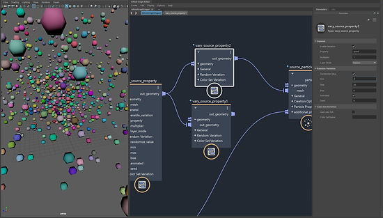

Turbulence and Modifier Influence
The turbulence influence offers a curl noise acceleration, which is useful for effects like air turbulence. A nice feature of the curl noise is that the resulting velocities are incompressible, like an air flow, which results in more natural particle smoke simulations. In such cases higher drag values will help the particles to more closely follow the curl noise flow instead of building up velocity over
The modifier influence can be used to replace, add, multiply or clamp the value of a simulation property like voxel_density,point_velocity, or point_size.
To use this node, plug its output into the influences input of a simulate node like simulate_aero, simulate_particles, or simulate_mpm.
Below is a screenshot with how my bifrost graph looked after creating the particle simulation

Arnold renders for my simulation:


WEEK 4
Bifrost Graph Aero System
This week we learned about the smoke effects in Maya using the Bifrost graph aero system.
Maya Fluid Effects is a technology for realistically simulating and rendering fluid motion. Fluid Effects allows us to create a wide variety of 2D and 3D atmospheric, pyrotechnic, space, and liquid effects. We can use the Fluid Effectssolvers to simulate these effects, or we can use fluid animated textures for more unique, distinguishing effects.
Our task today was to create a smoke effect. When I first created it, the smoke just rised and developed a sort of mushroom cloud. We started by adding a node called simulate aero.
I added a Torus Polygon and connected to the collider node. Collider is an obstacle to the flow of a Bifrost simulation. Today, I used it to form a barrier around the smoke.

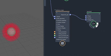
Source Air
Air Properties:
-fog density:
-
set: Sets a source into a property (note that if edges are hard in the input, this will also be the case in the output).
-
rate: Blends and adds a source as a time-dependent rate into a property.
-
add: Blends and adds a source into a property.
-
subtract: Blends and subtracts a source into a property.
-
over: Blends a source into a property.
-
min: Blends based on the minimum of the source and the property.
-
max: Blends based on the maximum of the source and the property.
-
multiply: Blends based on the product of the source and the property.
- initial_speed: The initial speed (velocity magnitude) of properties emitted.
-initial_speed_direction: The initial velocity-direction of properties emitted.
- speed_mode: How initial_speed, initial_speed_direction and inherit_velocity is emitted into voxels. The options are the same as for fog_density_mode.
-inherit_velocity: The proportion of the source geometry's velocity added to the velocity of properties emitted by the source. When using a vary_source_property node to randomize inherit_velocity, the value of inherit_velocity must be set to the smallest number used in the randomization to get a smooth trail in the presence of negative inherit_velocity values.
-trail_smoothness: The smoothness of smoke emitted in the presence of large source velocities. If the emitted trail of smoke has too much noise or obvious holes, trail_smoothness can be increased in increments of one to reduce such artifacts., On the iterate compound inside source_air there are some additional controls that can come in handy to ensure smooth emission in the presence of large velocities and/or large negative or positive inherit_velocity values
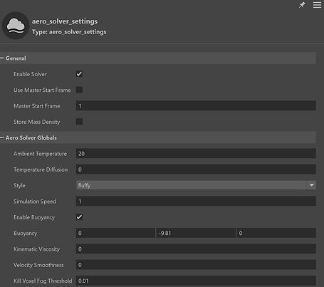
Aero Solver Settings:
ambient temperature: the temperature from
temperature diffusion: how much temperature will dissipate in the air
style: we got different styles of smoke
Accuracy: how many times the simulation will calculate a frame


Assigning Material:
Steps:
-add assign material node into the graph
-connect file cache (out object input) to assign material (geometry) and then assign material (out geometry) to output( out objects)
-create material into the hypershade then middle mouse drag it into graph and plug it into material
-in attribute editor on material change the name of the channel and replace it with the specific ones on bifrost property
-turn the color emission off


Vary Source Property:
This compound is useful to set per-point values on simulation sources. For example we could use this compound to vary the size of the points generated in a particle simulation.
The compound can vary the source property randomly or using a color set that exists on the input geometry in the scene.
Into property box, I wrote 'fog_density' and set the layer mode to replace. Finally I added random values into min and max.
Then I created another vary source but this time for temperature, speed and direction
Influences:
-> Vorticity influence: This applies vorticity confinement to the velocities of a simulation. This helps encourage small scale vortices in the simulation that might get otherwise damped. It will make the simulation appear more turbulent and less viscous.
->Modulate influence: The modulate_influence node varies the effect of an influence based on another property
Rendering:
->we can increase the samples and volume samples from skydome light up to 2 or 3 in order to get rid of the noise
In render setting ->ray depth ->volume (it offers soft light and volume when it's increased to 1 or 2)
WEEK 5
Bifrost Graph Combustion Aero System
This week we looked into combustion aero system.
Set up:
-first, we added a basic combustion graph and exploded it
-the temperature we set in air properties (source_air) needs to be high enough to ingnite the fuel temperature into source_fuel
-change from relative to absolut the resolution from source air
-in air properties: speed, temperature and fog need to be set up to set mode
-add the file cache node
-assign material by creating AiStandardVolume into hypershade and then bring it into the graph; write down into density channel 'voxel_fog_density'; emission needs to be changed to blackbody and into emission channel is 'voxel_temperature' as well as into temperature channel
Vary Source Properties
-we can use the vary source properties from the smoke simulation by grouping them into a compound and then publish them into Autodesk->Bifrost->Compound


Fuel settings:
-fuel type allows us to match real world footage if we now the type of fuel
-ignition temperature: The temperature at which the fuel ignites in degrees Celsius. Below the ignition temperature, no combustion takes place. Note that each type of fuel has a real world ignition temperature, but it can be re-defined here for artistic purposes.
-oxygen percentage: The percentage of oxygen in the oxidizer. For example, if oxygen_percentage is set to 0.4, the oxidizer will consist of 40 percent oxygen and 60 percent nitrogen. Typically, if there's sufficient fuel, increasing oxygen_percentage will lead to more violent explosions, increased flame propagation speeds, and higher temperatures.
-burn rate: A value between 0 and 2 that defines the stoichiometry of the mixture of fuel and oxidizer. A value of 0 leads to a smoky flame and more specifically means that only fuel will be emitted. Values below 1 correspond to fuel-rich conditions where there will be excess fuel after the combustion process. Increasing values from 0 to 1 gradually transition the simulation from a smoky flame towards a cleaner but also more violent combustion. A value of 1 indicates perfect stoichiometric conditions, that is, all available oxygen and fuel will react to form by-products with no excess oxygen nor fuel. Values above 1 correspond to fuel-lean conditions where there will be excess oxygen after combustion.

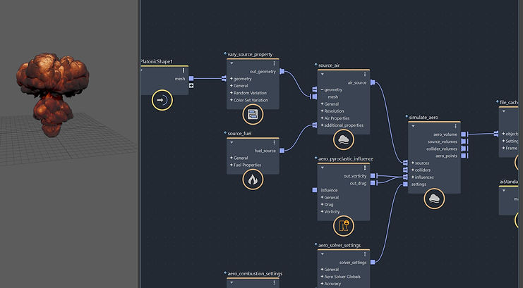

Aero Combustion settings
Thermodynamic properties-> Expansion -> makes the explosion bigger when increasing it
Radiative heating ->how quickly the heat passes through the atmosphere


Assignment 1
Bullet Rigid Bodies and NCloth
For our first assignment, we had to complete 2 tasks: to demonstrate destruction using Bullet Rigid Bodies and to demonstrate the movement of clothes using NCloth.
For the first task, I decided to use Jenga and to realize the destruction with the help of the ball. I created the jenga tower in Maya and applied bullet rigid body.
To the jenga pieces, I applied initially sleeping and linear damping so they will not move before animation starts. Collider shape will be box. I also applied bullet rigid body (mesh->static mesh) to the floor (a plane). Then, I created the ball which has the kineatic type. However, for the animation to make more sense, I added dynamic type until the ball hits the jenga tower, and then I keyframed it to be kinematic and one frame forward dynamic again.
I played around with translate rotate attributes until I managed to recreate the movement from my reference.
I increased the mass of the ball so it will have more impact. Internal fixed frame rate will be 120Hz.


When I was happy with the animation, I worked on creating a simple environment. I textured the ball, jenga pieces and the walls and the floor. However, the animation was wrong in the render, because the pieces were going through one eachother. The problem was the displacement material, so I had to remove that.
Then, I created a camera and added skydome light. I used a hdri image and I turned the camera visibility off.


NCloth
For the second task, I decided to film a pillow sheet falling over a desk and recreate it in Maya. I created a plane with 40 subdivisions and applied NCloth. On the desk and floor I applied passive collider. I tried applying a preset but nothing was really fitting as I wanted, so I decided to work from scratch.
It took me a lot of time to achieve the same movement as in the reference. For this, I adjusted mostly the strach resistence, bend resisteance, rigidity, damp and strech damp.


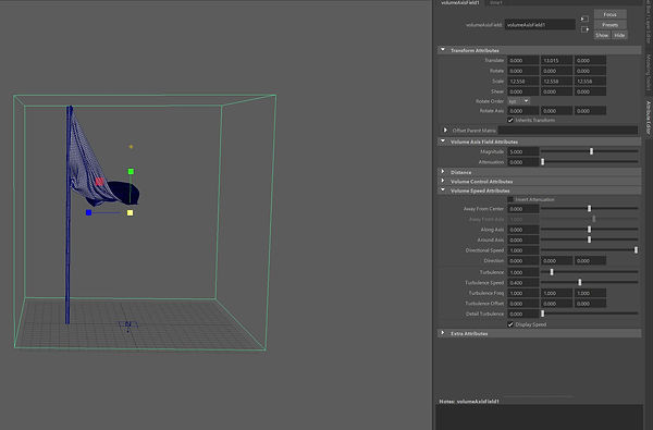
Then, in order to make the animation look more real, I went to fields-> volume axis. I did this in order to apply wind on ncloth so that it will move on its way down. I adjusted the position of the volume axis to look exactly as in the reference. Then, I played around with direction, direction speed, turbulence and turbulence speed.
Finally, I created a simple environment and textured models. Then, I created a camera and added skydome light. I used a hdri image and I turned the camera visibility off.

Final Result Assignment 1
WEEK 8
Bifrost liquid introduction
In week 8 of the module, we have been introduced to Bifrost liquids. We looked into scene scale, kill plane and how to cache liquids. Finally, we learned what is the best way to render liquids. First, we went to Bifrost fluids->liquid to apply the liquid effect into the shape we added into the scene. We had to change the scale of the liquid in cm, so we changed the gravity to 980 and the physical density to 0.001


As the liquid was overflowing beyond the ground plane, we had to use a kill plane. By doing this, the simulation stops when it goes beyond the kill plane. Another essential thing to do, is to use motion field and to play around with its attributes such as noise, turbulence, density, etc in order to get the best result regarding how the liquid moves.
Drag: more drag, the quicker the liquid velocities are effect by the motion field
Normal drag effects the motion of the liquid, good for breaking up the flow


Results of changing the resolution values:

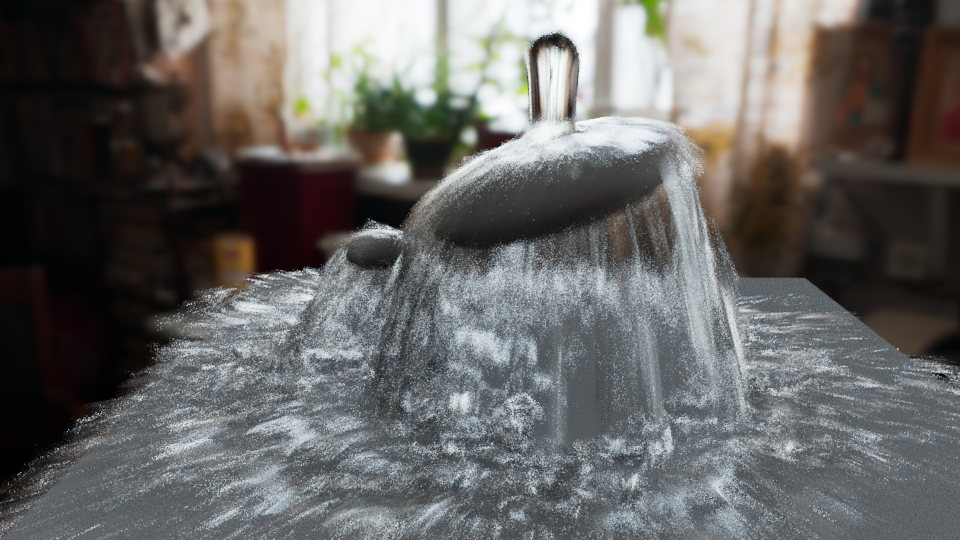
MY FINAL RENDERS

WEEK 9
Bifrost Ocean
In week 9, we continued to explore Bifrost fluid system. Our task was to create an ocean that will mimic reality as much as possible. We started with a plane, and we added Bifrost Ocean Modifier to it, which will create a sea type of plane. We looked into the attributes and played around with them to see how can we make it more realistic.
I created a cube and went to bifrost->liquid. Then, I set an emission region which was another big poly cube that will cover most of the ocean. I looked into death age and blend with guide.
Death Age (emission region only)
Length of time in seconds that a particle can be outside its emission region before it is deleted.
Blend With Guide (emission region only)
The blend weight of the input velocities from the guide. This helps to provide a smooth transition from the simulation to the guide.

In order to create a splash, I used a sphere that I animated to hit the water then I selected it along with the bifrost liquid, and created it a collider. When I was happy with the results, I cached it. Then, I added a killplane to bifrostemission region.
Next step was to create foam by selecting the liquid and clicking on bifrost->foam. Then, I played around with foam attributes to obtain a cool effect.
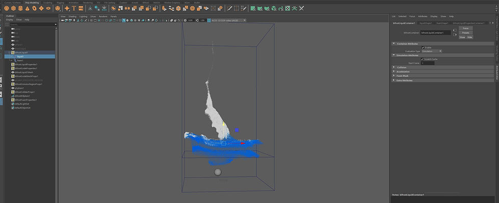
After changing some of the settings of bifrost meshing, I have exported the mesh as alembic. Then, by selecting the liquid, I imported the alembic cache.

REDERING TIME
Finally, I added a hdri image on the skydome light and I added material on water. For BossOutput (ocean) I created an aiarnold standard surface material with deep water preset, where I played around with depth (transmission). I added another material on bifrostliquid mesh. We need to turn on export vertex colors on export (BossOutput). I created ramp as projection (geometry) on BossOutput material in order to get a wave type of effect. I chose circular ramp, smooth type, and I turned off Wrap U and V.
On color balance(ramp), I set the default color all the way up.

REDERS AND PLAYBLAST


WEEK 10
Bifrost Graph MPM
The material point method (MPM) is a numerical method used to simulate a wide variety of substances, like snow, sand, and cloth. All these materials use the same simulate_mpm node, so they can be combined and interact with each other in the same simulation.
MPM can also be used to simulate materials like fluids and fibers, but these are still experimental in Bifrost
We explored MPM by working on a scene that included a snow mesh, sand mesh, cloth mesh, and water mesh; pit mesh is collider
Setting up the graph:
-Simulation->MPM ->simulate mpm
-create mpm solver settings
-simulate mpm->source->create node->add all the sources (snow, sand, cloth, pit, water)
Starting with the snow
-add mesh into geometry
-source mpm snow->additional properties-> set property (k=color, math float 3)
Repeating the same process for all emitters
-add a collider and connect it to pit mesh; collider connected tro colliders (simulate mpm); resolution: absolute
-connect granular particles, volume and cloth mesh to output


We then looked into the attributes of mpm snow.


We continued to look into mpm sand

source mpm fluid

cloth and tearing


After I played around with the attributes for all the emitters, I started caching. Then, I made a playblast render.
We then learnt how to split the sources into separate outputs.
-assign material (connect out object from file cache to geometry and out geometry to out objects from output)
-create the actual texture in hypershade, bring it into the graph, connect material reference (from texture) to surface material (assign material)
-add split points by material; connect granular particles (simulate mpm) to points; connect fluid particles to objects (file cache)
-repeat the process for all emitters
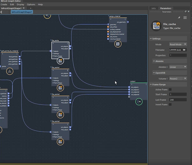

Converting to mesh
Snowball hitting a wall
For the next exercise, I created a snowball hitting a wall. Below are some screenshot with my bifrost graph and the parameters.


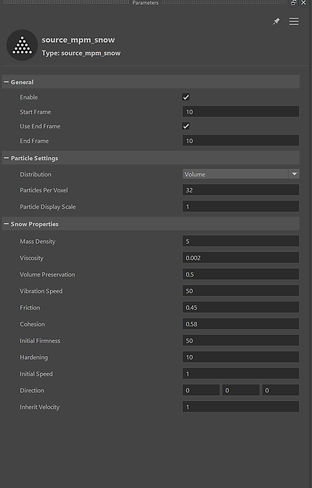


Final Animation
WEEK 11
Bifrost Strands
This week we learnt about strands. To begin with, we created a simple strand just by using the bifrost graph. We looked into the basic settings and applied aiStandardHair material.
Introduction to Strands


Next, we used a platonic shape to start with and created strands on it. We looked at strands along normals
We used f curve to adjust how the strands are moving.


By applying colorseteditor, we only marked with white color what we wanted to render in Arnold.


Particle Strand Trails:
In the next exercise, we learned how to create trails with strands. We generated strands from a geo such as a plane. We then get the points from the plane to generate the trails. Below are my renders after using this method.


WEEK 12
XGen Hair
This week, we created XGen hair in Maya. So, we used a head model to apply hair to it.
Basic Set Up
-make sure we detached the area where we are applying the hair (otherwise the hair will generate over the whole surface)
-generate-> Create XGen Description ->Placing and shaping guides need to be on
Setting Guides
-we started applying hair and giving it a shape by moving the vertexes
-XGuide Shape-> Primitives ->Rebuild Guide
-we get more hair if we bump the density up
-modify CV Curve and spline segments need to be increased as well

Guides Clumping
XGen -> Sculpt Guides
After adding clumps, we can add noise as well, where we should set the magnitude a bit down


Rendering and Caching
First, we need to apply a shader on ->aiStandardHair
-melanin will change the hair color
-we can also play around with roughness, randomize melanin, etc
We can also cache the hair out if we want to apply it to animation later on
hairSystemOutputCurves -> Cache ->Alembic ->Export Selection to Alembic
Then, cache->import alembic
Now, we can animate the head turning and the hair will follow its movement


Grass Collision
For the next exercise, I started with a plane that is sliding down. Then, I added a sphere and applied a bullet->dynamic rigid body on it. The Plane will be a static body. This will animate the sphere. I also baked the simulation.

Interactive Groom Editor
Before creating the groom, we need to get rid of the bullet.
I increased the taper, scale, and density multiplier. I added a noise multiplier.

Applying shader
I assigned aiStandardSurfaceHair material on grass. On the plane I added aiStandardSurface and on weight, I applied layered texture and noise (2d Texture on alpha)
In order to view in in Arnold, we need to set melanin and melanin redness to 0


Collision Modifier
Because on my machine, in collision tab, collision object was not showing any attributes, I had to apply the collider in the node editor, which seemed to work just fine. Finally, I just played around with some attributes in the Groom Editor such as scale or collision modifier mask

Final Render
From my last year's experience when I created fur for my cat model, I know that fur takes a lot of time to render and it crashes often, so I only rendered 1 frame. I increased 'camera' and 'specular' in Arnold Render Settings.

WEEK 13
Bifrost Instances
This week we looked into instances using Biforst
What are instances?
Instances are copies of geometric objects placed at the positions of points, such as the points of a particle system. Instances result in lighter scenes because only the master geometry and the points need to exist. Instances can be used to create trees in a forest, objects falling into a pile, and much more.
Instances work by associating points with an instance shape, which consists of geometry plus additional information such as an optional preview geometry to use for display in the viewports.
Create Instance Node
Starting with a plane and 5 shapes, I brought 5 different types of meshes and I connected them to 'create instances' node. The 'create instance' node allows the meshes to align on the plane. I added 'scatter points' node to randomize the meshes
'randomised point scale/translation/rotation' node can change the meshes' direction or scale randomly.
Randomise Points (SRT)
We can also randomize the instances, such as their scale, rotation, and translation with 'randomise point rotation'.


Randomise Selection by Probabilities


Allocation of shaders to instances
If we want different shaders for meshes, we need to allocate them before instances.
I applied aiStandardSurface material as well as noise and displacement map.


Lego Man
In the next exercise, I used a 'Lego Man' mesh and applied the 'create instance' node on it. I exported the lego model as an ASS file and imported it back with Standin. Next, I created a cube having the size of the lego and connected the 'preview_geometry' pipe on the Render Archive Instance.


Different Color Hat
In order to achieve different color hat, I used the operator selection:/legoToy:C_legoToy01_low/legoToy:C_legoToyHat_low/*
I created aiStandardSurface material, and connected aiUserData to base color in order to change the color of lego toy hat. On property, I added 'aiSetParameter' and shader. Next, I applied the material node into the shader, dragged the material into bifrost graph and connected the operation.
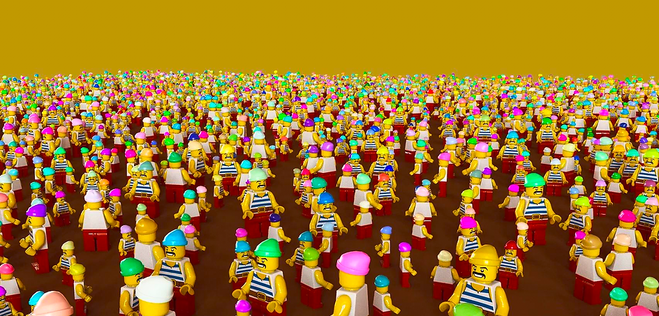
Assignment 2
For the final assignment, we need to create three different real-rendered environmental effects scenarios using Bifrost simulation from Autodesk Maya software. These scenarios will be defined by these three titles:
-
Natural – Simulated environmental effect mimicking a natural phenomenon that occurs in the world. Examples - are rain, wind, fog, fire, or shooting stars.
-
Fantasy Sci-Fi - Simulated environmental effect that has a fantasy or science fiction element. Example – Wormhole or glowing magic cloud.
-
Surreal - Simulated environmental effect that has an odd or unexpected element. For example – Diamonds cover every surface in the scene.
01-Natural
For the natural assignment, I created a physically accurate ocean using BOSS editor.
Starting with a plane, I first added a boss spectral wave for which increased the resolution and the patch size.
Waves are a result of wind and ocean depth, so I adjusted wind speed and Fetch Distance as well. I turned on the horizontal displacement and increased the wave size. For more accuracy, I created a second wave. Then, I applied aiStandardSurface material and added the deepwater preset


Creating Foam
I turned on foam generation on the first wave and cached it. I assigned the cache in the AIsurfaceshader, emission tab to be able to see foam in the render. As it can be seen below, I got too much foam so I had to reduce Cusp Min value


Adding Displacement Map as Projection
I increased the patch size and then played around with wave size.
Finally, I added a new plane, applied the existing ocean shader to it, and on the displacement material I added as projection which produces a place3dtexture in the scene. I rotated it so it points down and scaled it to half the patch size. Then, I added the wave cache. I repeated the process for the second wave.

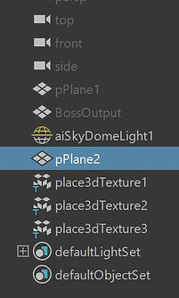

I changed the subdivision type, which means that at render time, Arnold will subdivide each face again (3 times)

Adding a boat wake
Finally, I downloaded a boat model which I added to the scene and animated it. I created a WaveSolver. I made the boat 'geometry influence'. On bossgeoproperties tab, I played around with amplitude


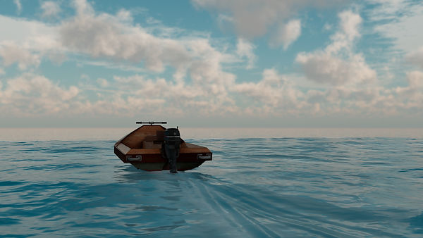
Adding dynamic foam
First, I added bifrostLiquid. I set the boat as EmissionRegion. I changed the masterVoxelSize to 0.1 (liquid container). The smaller the voxel, the more particles we can fit in a small place. In order to generate the particles just outside the boat, I increased the thickness on EmissionRegion. Then, I added a Guide and Foam.
I played around with foam attributes such as particles, min liquid speed, and curvature. I deleted the liquid, and kept only the foam.
Rendering Foam
To get an accurate result when rendering the foam, I change the ray depth -> volume to 4, in Arnold Render settings. I set the emission mode to density on aiStandardVolume (foam texture)


01-Natural: Final Renders


02-Fantasy
For the fantasy assignment, I created a colorful growing shape made of particles. I did this by scattering points in volume and making their movement driven by aero volume.
Starting from a mesh sphere, I converted it into a volume. Then, I played around with 'scatter points' attributes.
I added 'create_instances' to create more spheres
'Sample Volume' (property: voxel distance value) will produce the distance value for each point.
I connected 'Sample Volume' to 'Change Range', to get different values for points.
Then, I added 'Set Geo Property' to play around with points' size (property: point_size)


Aero Volume
I set up an aero simulation and for each frame, I used the voxel velocity to drive the displacement of particles. I assigned an aiStandardVolume material. On the aero simulation, at source_air, I changed the resolution mode to 'absolute', I played around with fluid size and geo detail size.
source_air ->fog density mode: set
I added initial speed and direction (along the y-axis)
aero_solver_settings ->style->fluffy
I got a 'vary_source_property' (property:fog_density) to obtain a variation of fog density
Influences:
'vorticity_influence' and 'drag_influence' to make it more dynamic
'modulate_influence' to create more variations.
Then, I added more influences such as dissipation


Driving Particles' Movement with the Aero Volume
I set up a 'simulate particle solver' and applied a voxel velocity as an influence
'Volume_particle' will make the particles follow the aero volume. I had to increase the force scale to get an accurate result.
I added 'drag_influence' to dampen the velocity
'Set_geo_property' (property: color) to assign colors to the points


Getting color variation
I applied the colors based on the magnitude of the voxel velocity. 'Sample_volume' gets the voxel velocity where particles are located and 'get_point_position' gets the particle position( Math: float3 for value). Then, I got the lengths of the vectors with 'length'
'Evaluate_fcurve' is essential because it helps at modifying the change range using a curve.
'Lerp' calculates the interpolation between 2 colors


Final Bifrost Graph:


Assigning texture and caching


.png)
02-Fantasy: Final Animation
03-Surreal
For the last part of the assignment, I created a man that transitions into chunky spheres, then collapses, using a 3d model from Maya Content Browser and motion capture.
Character Set Up
I made an alembic cache of the animation running and I baked out the shader as a vertex color (single image).
To do this, I added a light then I went to utilities-> render selection to texture, with a 2048 resolution and I baked it out.Then, I applied the running mocap to the character and exported the alembic (I turned on UV write and UV set)

Bifrost Graph
I made a 'simulate_mpm' in which was going a source for snow, a collider which is represented by the plane, and the 'mpm_solever_settings' (with a detailed size of 0.06). On 'mpm_solver_settings' I changed the shape to spheres.
I set the collider to Absolut and Shell.
'Source_mpm_Snow':
-increased particles per voxel
-played around with friction, cohesion, initial firmness
-direction is set to :0, -1, 1 so he is falling down
I wanted the Bifrost to only start at frame 33, so, in the channel box, I turned off the visibility of the mesh at frame 33, and at snow_mp_source I enabled the start and end of frame 33.
Finally, I duplicated the plane and made it smaller. So, I have a collider plane and a render plane. I moved the collider plane as in the screenshot below so that the subject will fall forward.


Getting colors in the viewport and Assigning material
Adding Color Set
With the mesh selected, Display->color set editor-> make a new color and call it 'color'. I made it an RGBA, but it was easier if I was doing an RBG because I don't need the alpha after all :)
The next step was to get rid of the alpha. In order to do this, I created a 'vector4 to vector3' node. I named the 'Get_geo_property' node 'color' as well.
Finally, I created an AiStandardSurface material and an aiUserDatacolor(renamed: color). I connected 'outcolor' (of 'userdatacolor') to the base color and subsurface color of the standard surface.


03-Surreal: Final IMG Render and Animation

WEEK 14
Extended Bifrost Work
In the last week of the module, Jason taught us how to create some more cool stuff using Bifrost Graph, in Maya.
First, we generated points using 'construct_points'. As usual, we randomized their scale attributes such as translation and their colors.

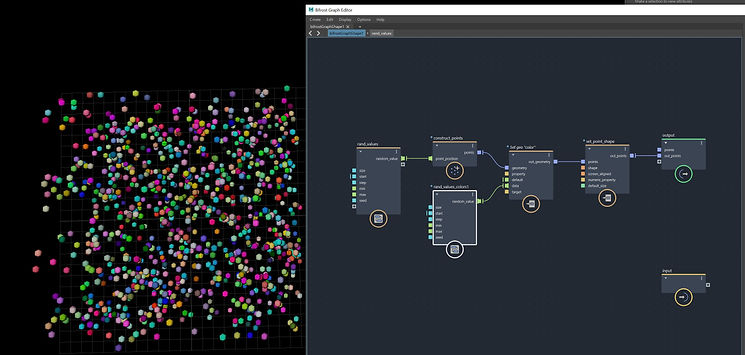
To assign the points different values on different frames, we added 'rand_values' and applied an 'if' condition. We randomized their scale and color


Finally, we brough a plane into the graph editor and connected it with 'fractal_turbulence field' and 'vector_field_scope'


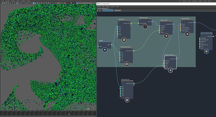
Final Renders


Further study and optional exercises
Particle Trails
My aim was to create a fairy particle trail. I started with a sphere which I animated to rotate up to the value of 360 and to move in the Y axis. I applied Emit from Object, having points selected. Then, in order to make the trail more visually engaging, I played around with different attributes of the emitter and of the nparticle as can be seen in the screenshots above. The most important ones were lifespan and turbulence.


Final Renders


Playblast
Flame
I created a flame using Maya Fluid. I adjusted the turbulence on the emitter and increased the base resolution of the fluid. I played around with different attributes such as density, temperature, and color. I turned auto-resize on.


I added Fluids ->Emitter and set a key on its Y axis and I moved it up. When I was happy with the results, I added an area light and a skydome light. I tried to make the smoke blue so it will be more interesting. To do this, I went to fluid->shader->color, and played around with color and opacity values.


Final Render

Playblast
Aero Bifrost
I started with a sphere that I modeled in a weird shape by selecting the vertexes with the help of the soft selection tool. I then animated it. I applied Bifrost fluids->aero and motion field. After adjusting the temperature, turbulence and scaling down the master voxel size to 0.100, I cached it.

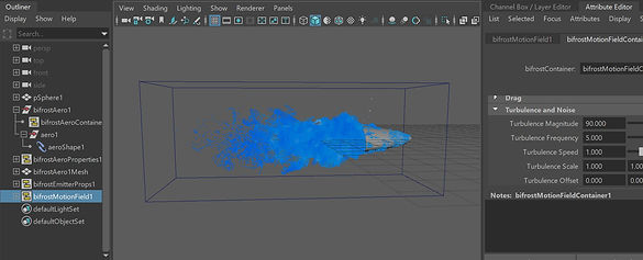
Applying Material
I assigned aiStandardSurface material and connected aiUserDatacolor. The property for userdatacolor was velocity. I adjusted few attributes, then I added colorcorrect node. I increased the hueshift up to 200 to get a varierty of colors. Then, I created few torus shapes around my aeroshape for which I assigned standardsurface with metalic preset. In order to view the result in Arnold, I added skydomelight and set the exposure to -3. I kept changing the size of the points to see what I can get.


Final Renders


